Long wire antenna for portable operations.

With the view to establish a quick and easy multi-band antenna for portable and camping operations a simple long wire antenna with an earth or earth plus counterpoise arrangement with a 9:1 voltage unun including a tuner or simply with a tuner is one possible solution. With the 9:1 voltage unun and wire lengths suggested in the below tables the antenna should present non extreme impedances for all HF amateur band frequencies. This page is far from complete and represents the ongoing investigation into this type of antenna. Experiments to date seem to have raised more questions than obvious answers. 

Description

The ARRL Antenna Book describes the general characteristics of Long Wire Antennas. Whether the long wire antenna is a single wire running in one direction or is formed into a 'v'. rhombic or some other configuration. there are certain general principles that apply and some performance features that are common to all types. The first of these is that the power gain of a long wire antenna as compared to a half wave dipole is not considerable until the antenna is really long (its length measured in wavelengths rather than metres of feet).

While the below described antenna does not fit the criteria for a true long wire antenna on the lower bands it will on the higher band above 20m and certainly meets the definition at 10m. Technically a true "longwire" needs to be at least one wavelength long. but Hams commonly call any end-fed wire a longwire or more correctly random wire antenna.

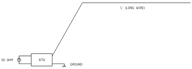
Figure 1  Typical ATU and long wire antenna configuration with an earth or earth plus counterpoise. 

Figure 2  Typical 9:1 voltage unun and long wire antenna configuration with an earth or earth plus counterpoise.

The feed impedance of the end fed long wire antenna is perhaps the main consideration particularly as in this case the antenna is to be a multi-band antenna, being a useful radiator on all amateur radio bands from 80m through to 6m. If the antenna were to be a single band antenna with the wire cut to a ¼ wave length at the desire frequency this would produce a feed impedance somewhere between about 30 ohms to 80 ohms and would therefore be relatively easy to achieve a useful match. A multi-band end fed wire antenna presents a potential problem in that a ¼ wave length antenna cut for say the 80 metre band will present a feed impedance of about 70 ohms however when the same antenna is used on the 40 metre band the feed point impendence will be several thousand ohms and therefore difficult to achieve a match even with a quality tuner. The trick is to making this type antenna an easier match by avoiding the lengths that are 1/2 wavelength and harmonically related to 1/2 wavelengths or simply multiples of 1/2 wavelengths that will present the most extreme rang of impedances. Figure 3 is a table of lengths to be avoided in relation to spot frequencies within all amateur HF bands and including the 160m band and 6m band, the lengths are 2% shorter due to the real world effect of the wire diameter. The values in Figure 3 have been determined with the following simple formula to determine the 1/2 wave length of wire for a given frequencies of interest and multiplied across the table to determine the harmonic related lengths.  

The Figure 4 scatter graph presents the data from the Figure 3 table showing blue dots for the lengths of wire to be avoided in vertical as related to frequency in the horizontal. For example a wire length of 45m metres projected across the scatter graph does not intersect with a blue point and is in fact well clear of any dots making it an ideal wire length.

Figure 3  Table of wire lengths 'L' in metres to be avoided based on multiples of 1/2 wave lengths of popular amateur radio frequencies.

Figure 4  Scatter graph of wire lengths 'L' in metres to be avoided based on multiples of 1/2 wave lengths of popular amateur radio frequencies.

Based on conclusions from Figure 3 & 4 tables a length of 12.87m chosen

The graph in Figure 5 has been produced with data generated from 4NEC2 antenna modelling software for a wire length of 18.7 mtr. The modell was to determine installation effects on the  impendence distributed over a frequency range from 1 MHz through to 30 MHz. The modelling assumes good ground conductivity and all antenna configurations have a modest 4.0 mtr counterpoise, remembering that the objective of this exercise is to evaluate a simple easily deployable portable multiband antenna.  

The details of the three antenna configuration modelled with 4NEC2 are as follows;  

·         An antenna wire of 18.7 mtr in total length with 15.7 mtr installed horizontally at 2.5 mtr above the ground and with a 3 mtr 30 degrees angled lead in section to the RF source or the graphed impedance load point.

·         An antenna wire of 18.7 mtr in total length installed at an angle of 30 degrees from the RF source or the graphed impedance load point.

·         An antenna wire of 18.7 mtr in total length installed at an angle of 60 degrees from the RF source or the graphed impedance load point.

·         An antenna wire of 18.7 mtr in total length installed vertically from the RF source or the graphed impedance load point.

While these four configuration are the extremes for this type of antenna installation it is interesting and surprising to note that while there is some effect on the location of the high and low impedance nodes in relation to the frequency it is not as dramatic as I would have imaged. Also worth noting that the range of impedances ranging from near 5k ohms to less than 100 ohms should be within the range of any reasonable antenna tuner however the data samples for the graph were generated in 0.5 MHz intervals and smoothed with the result that the peaks at 8 and 16 MHz and trough at 5.5 MHz may be more extreme than the graph suggests.

Figure 5 Produced with data generated from 4NEC2 antenna modelling software. Four variation of a random wire antenna with a length of 18.7 mtr.

The graph in Figure 7 has been produced with data generated from 4NEC2 antenna modelling software for an antenna wire of 18.7mtr total length installed at an angle of 30 degrees over a selection of ground types. Despite ground types all graphed impedances peaks and troughs are at roughly the same frequencies with the only clearly noticeable shift being over perfect ground which is obviously not likely to be encounter. These ground types represent the extremes with most if not all real world types falling within the ranges presented.

4NEC2 antenna modelling software ground definitions.

Figure 6 Produced with data generated from 4NEC2 antenna modelling software for an antenna wire of 18.7 mtr total length installed at an angle of 30 degrees over a selection of ground types.

All very interesting until the assumptions and modelling were developed into a practical antenna following the parameters established from the modelling. The results shown in Figure 7 with data generated from an AIM 4170C antenna analyser were very interesting as the results varied dramatically from the model in every respect, while the values of the impedance peaks and troughs were expected to vary its was completely unexpected that the peaks and troughs were so far out of alignment in terms of frequency. The first trough at approximately 5.9MHz appeared at 4.0MHz and at about 25% of the value in the real antenna. The first high impedance peak within the HF band was around 8.1MHz in the model and 6.6MHz in the real antenna.  

Attempting a bit of relatively blind experimenting, a 4.3m length was added to the wire antenna bring it to a new total length of 23m. 

The results shown in Figure 8 with data generated from an AIM 4170C antenna analyser of the new 23m radiator are an improvement of sorts, however the feed impedance over the 1.0 - 30MHz spectrum have changed to the point of being unrecognisable with respect to the slightly shorter 18.7m radiator. 

Figure 9 shows the continuing unpredictable nature of this antenna with the addition of the 1:9 voltage unun at the feed point producing a graph of the impedance that seem to have little in common with the antenna without the unun.

Figure 7 Measured impedance from 0.5MHz to 30MHz of the 18.7mtr total length end fed wire antenna. Graph generated with data from from an AIM 4170C antenna analyser. The three parallel red lines indicate the range that it was hoped that most amateur bands would fall into.

Figure 8 Measured impedance from 0.5MHz to 30MHz of the 23.0mtr total length end fed wire antenna. Graph generated with data from from an AIM 4170C antenna analyser. The three parallel red lines indicate the range that it was hoped that most amateur bands would fall into.

Figure 9 Measured impedance from 0.5MHz to 30MHz of the 23.0mtr total length end fed wire antenna with a 1:9 voltage unun installed. Graph generated with data from from an AIM 4170C antenna analyser. The three parallel red lines indicate the range that it was hoped that most amateur bands would fall into.

Figure 10 Radiation plot for the 80m band were produced using NEC based antenna modeller and optimizer 4NEC2. Due the the short radiator this band dose not produce very efficient radiation pattern.

Figure 11 Radiation plot for the 40m band were produced using NEC based antenna modeller and optimizer 4NEC2. 

Figure 12 Radiation plot for the 30m band were produced using NEC based antenna modeller and optimizer 4NEC2. 

Figure 13 Radiation plot for the 20m band were produced using NEC based antenna modeller and optimizer 4NEC2. 

Figure 14 Radiation plot for the 17m band were produced using NEC based antenna modeller and optimizer 4NEC2. 

Figure 15 Radiation plot for the 15m band were produced using NEC based antenna modeller and optimizer 4NEC2. 

Figure 16 Radiation plot for the 12m band were produced using NEC based antenna modeller and optimizer 4NEC2. 

Also see  1:9 voltage unun

References 

The ARRL Antenna Book.

http://en.wikipedia.org/wiki/Random_wire_antenna

http://www.aa5tb.com/efha.html

The above radiation plots were produced using NEC based antenna modeller and optimizer 4NEC2by Arie Voors. The Antenna Analyser software can be found at http://www.qsl.net/4nec2/

TOP OF PAGE

Page last revised 13 November, 2024